There is a tool which is part of my Open Diapason virtual organ project called “sampletune” which is designed to allow sample-set creators to tune samples by ear and save the tuning information back into the sampler chunk of the wave file. The utility plays back a fixed tone and there are keyboard controls to shift the pitch of the sample up and down until the beats disappear. I was hoping to prototype a sawtooth wave as the tuning signal, but realised during implementation that creating arbitrary frequency piecewise-linear waveforms is actually somewhat a difficult problem - fundamentally due to aliasing… so I parked that idea and ended up summing several harmonic sinusoids at some arbitrary levels.
Recently, I was thinking about this again and set about solving the problem. It was only in the last couple of weeks that I discovered tools like Band Limited Impulse Trains (see link at bottom of post) which seem to be the common way of generating these signals. These are fundamentally FIR techniques. I approached the problem using IIR filters and came up with a solution which I think is kind-of interesting - please let me know if you’ve seen it done this way so I can make some references!
The idea
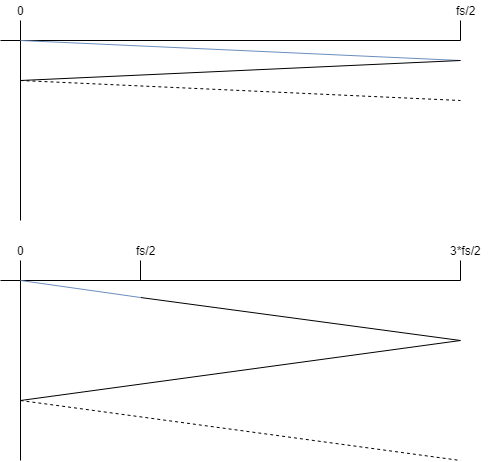
If we generate a piecewise linear waveform wave at a frequency which is not a factor of the sampling rate, we will get aliasing. In fact, we can work out the number of shifted aliasing spectrum copies which we can expect to see by taking \(f_0 / \text{gcd}(f_0, f_s)\). If \(f_0\) is irrational, we have an infinite number of copies. Let’s make the assumption that more-often than not, we are going to be generating a very large number of aliases. The next assumption we are going to make is that most of the signals we are interested in generating have a spectral envelope which more-or-less decays monotonically. With this assumption, we can say: if we generate our signal at a much higher sampling rate, we effectively push the level of the aliasing down in the section of the spectrum we care about (i.e. the audible part). Below is an image which hopefully illustrates this; the upper image shows the spectral envelope of the signal we are trying to create in blue, all of the black lines which follow are envelopes of the aliasing. The second image shows what would have happened if we created the same frequency signal at three times the sampling rate. The interesting content again is in blue and everything in black is either aliasing or components we don’t care about. What we can see is that by increasing the sample rate we generate our content at, we effectively push the aliasing components down in the frequency region we care about.
So let’s assume that instead of generating our waveforms at \(f_s\), we will:
- Generate them at a sample rate of \(M f_s\) where \(M\) is some large number.
- Filter out the high-frequency components above \(f_s / 2\) using some form of IIR filter structure.
- Decimate the output sequence by a factor of \(M\) to get back to \(f_s\) (which we can do because of the previous operation).
Now that we’ve postulated a method, let’s figure out if it makes any sense by answering the questions “does it have an efficient implementation?” and “does it actually produce reasonable output for typical signals we may want to generate?”.
Does it have an efficient implementation?
Denote a state-space representation of our SISO discrete system as:
\[ \begin{array}{@{}ll@{}} \hat{q}\left[n\right] & = \mathbf{A} \hat{q}\left[n-1\right] + \mathbf{B} x\left[n\right] \\ y\left[n\right] & = \mathbf{C} \hat{q}\left[n-1\right] + D x\left[n\right] \end{array} \]
For clarity, let’s just consider a single update of the system state where \(\hat{q}\left[-1\right]\) represents the “previous state” and \(x\left[0\right]\) represents the first sample of new data we are pushing in.
\[ \begin{array}{@{}ll@{}} \hat{q}\left[0\right] & = \mathbf{A} \hat{q}\left[-1\right] + \mathbf{B} x\left[0\right] \\ y\left[0\right] & = \mathbf{C} \hat{q}\left[-1\right] + D x\left[0\right] \end{array} \]
We can derive an expression to insert two samples in via substitution and from that derive expressions for inserting groups of samples.
\[ \begin{array}{@{}ll@{}} \hat{q}\left[0\right] & = \mathbf{A} \hat{q}\left[-1\right] + \mathbf{B} x\left[0\right] \\ \hat{q}\left[1\right] & = \mathbf{A} \hat{q}\left[0\right] + \mathbf{B} x\left[1\right] \\ & = \mathbf{A}^2 \hat{q}\left[-1\right] + \mathbf{A}\mathbf{B} x\left[0\right] + \mathbf{B} x\left[1\right] \\ \hat{q}\left[\sigma\right] & = \mathbf{A}^{\sigma+1}\hat{q}\left[-1\right] + \sum_{n=0}^{\sigma}\mathbf{A}^{\sigma-n}\mathbf{B}x\left[n\right] \\ \end{array} \]
\[ \begin{array}{@{}ll@{}} y\left[0\right] & = \mathbf{C} \hat{q}\left[-1\right] + D x\left[0\right] \\ y\left[1\right] & = \mathbf{C} \hat{q}\left[0\right] + D x\left[1\right] \\ & = \mathbf{C}\mathbf{A}\hat{q}\left[-1\right] + \mathbf{C}\mathbf{B}x\left[0\right] + D x\left[1\right] \\ y\left[\sigma\right] & = \mathbf{C}\mathbf{A}^{\sigma}\hat{q}\left[-1\right] + \mathbf{C}\sum_{n=0}^{\sigma-1}\mathbf{A}^{\sigma-1-n}\mathbf{B}x\left[n\right] + D x\left[\sigma\right] \end{array} \]
We’re interested in inserting groups of samples which form linear segments into our filter. So let’s replace \(x\left[n\right]\) with some arbitrary polynomial. This gives us some flexibility; we need only a polynomial of zero degree (constant) for square waves, first degree for saw-tooth and triangle - but we could come up with more interesting waveforms which are defined by higher order polynomials. i.e.
\[ x\left[n\right] = \sum_{c=0}^{C-1} a_c n^c \]
Let’s substitute this into our state expressions:
\[ \begin{array}{@{}ll@{}} \hat{q}\left[0\right] & = \mathbf{A} \hat{q}\left[-1\right] + \mathbf{B} a_0 \\ \hat{q}\left[\sigma\right] & = \mathbf{A}^{\sigma+1}\hat{q}\left[-1\right] + \sum_{n=0}^{\sigma}\mathbf{A}^{\sigma-n}\mathbf{B}\sum_{c=0}^{C-1} a_c n^c \\ & = \left(\mathbf{A}^{\sigma+1}\right)\hat{q}\left[-1\right] + \sum_{c=0}^{C-1} a_c \left(\sum_{n=0}^{\sigma}\mathbf{A}^{\sigma-n}\mathbf{B} n^c\right) \\ \end{array} \]
\[ \begin{array}{@{}ll@{}} y\left[0\right] & = \mathbf{C} \hat{q}\left[-1\right] + D a_0 \\ y\left[\sigma\right] & = \mathbf{C}\mathbf{A}^{\sigma}\hat{q}\left[-1\right] + \mathbf{C}\sum_{n=0}^{\sigma-1}\mathbf{A}^{\sigma-1-n}\mathbf{B}\sum_{c=0}^{C-1} a_c n^c + D \sum_{c=0}^{C-1} a_c \sigma^c \\ & = \left(\mathbf{C}\mathbf{A}^{\sigma}\right)\hat{q}\left[-1\right] + \sum_{c=0}^{C-1} a_c \left(\sum_{n=0}^{\sigma-1}\mathbf{C}\mathbf{A}^{\sigma-1-n}\mathbf{B} n^c\right) + \sum_{c=0}^{C-1} a_c \left(D \sigma^c\right) \end{array} \]
There are some interesting things to note here:
- The first output sample (\(y\left[0\right]\)) is only dependent on \(a_0\) and the previous state. If we restrict our attention to always getting the value of the first sample, we don’t need to do any matrix operations to get an output sample - just vector operations.
- All of the parenthesised bits in the equations have no dependency on the coefficients of the polynomial we are inserting into the filter - they only depend on the number of samples we want to insert (\(\sigma\)), the system state matrices and/or the index of the polynomial coefficient. This means that we can build lookup tables for the parenthesised matrices/vectors that are indexed by \(\sigma\) and the polynomial coefficient index and effectively insert a large number of samples of any polynomial into the filter state with a single matrix-matrix multiply and a number of scalar-vector multiplies dependent on the order of the polynomial.
It’s looking like we have an efficient implementation - particularly if we are OK with allowing a tiny (almost one sample at \(f_s\)) amount of latency into the system.
Does it work?
Below is a screen capture of Adobe Audition showing the output of a small program which implemented the above scheme. The system is configured using an elliptic filter with 1 dB of passband ripple and a stop-band gain of -60 dB.
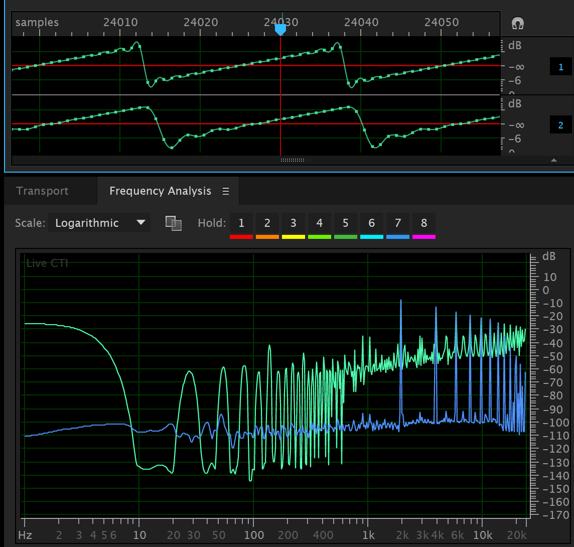
The waveform has a frequency of \(600\pi\) which is irrational and therefore has an infinite number of aliases when sampled (this is not strictly true in a digital implementation - but it’s still pretty bad). We can see that after the cutoff frequency of the filter, the aliasing components are forced to decay at the rate of the filter - but we predicted this should happen.
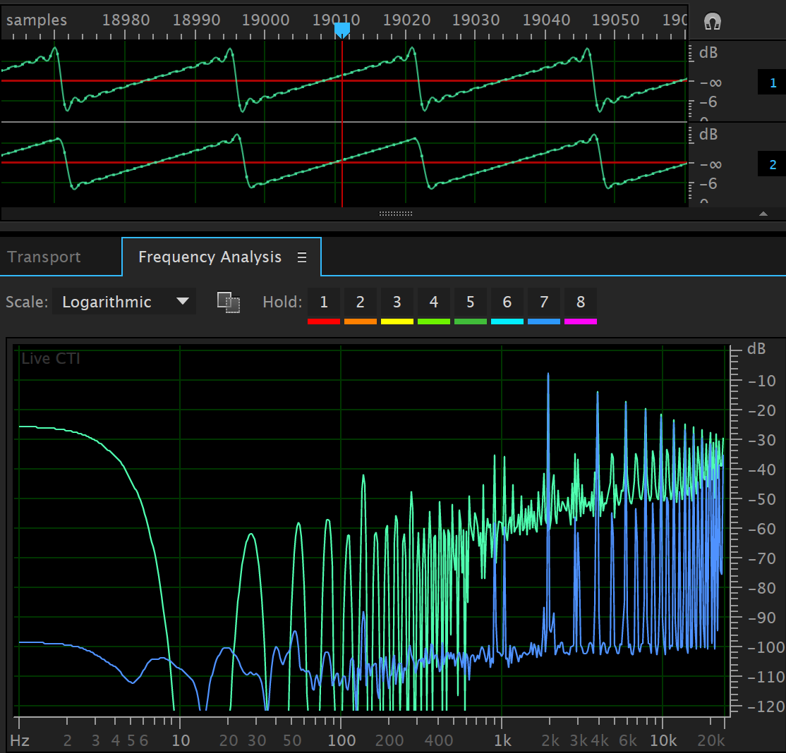
Below is another example using an 4th order Bessel filter instead of an elliptic filter. This preserves the shape of the time-domain signal much more closely than the elliptic system, but rolls off much slower. But the performance is still fairly good and might be useful.
Here is a link to a good paper describing how classic waveforms have been done previously Alias-Free Digital Synthesis of Classic Analog Waveforms, T. Stilson and J. Smith, 1996.