This is a tutorial on how to build a digital implementation of a 2nd-order, continuously-variable filter (i.e. one where you can change the parameters runtime) that has dynamic behaviour that mimics an analogue filter. The digital model is linear (i.e. we are not going to model any transistor/diode behavior - we'll do that in another blog). The resulting implementation is suitable for use in a digital synthesiser or equaliser. It is not attempting to be a perfect model - but it should be quite close.
The tutorial follows this rough guide:
- Difference equations and a recap on state-space.
- Description of the circuit we will be modelling (this can be skipped - it is included for completeness).
- Expressing the desired system digitally using a partially-transformed state-space model.
- Making the filter more useful
- Summary of implementation and demo video
Difference equations and state-space recap
Most EE grads know how to get a digital implementation of an analogue filter:
- Pick a transfer function and select values for the natural frequency (\(\omega\)) [rads/second] and the dimensionless Q-factor (\(Q\)) - these two controls are like the “frequency” and “resonance” knobs on a synth filter. \[ \begin{array}{cl} \text{Lowpass} & \frac{\omega^2}{s^2 + \frac{\omega}{Q}s + \omega^2} \\ \text{Highpass} & \frac{s^2}{s^2 + \frac{\omega}{Q}s + \omega^2} \\ \text{Bandpass} & \frac{\frac{\omega}{Q}s}{s^2 + \frac{\omega}{Q}s + \omega^2} \\ \text{Bandstop} & \frac{s^2 + \omega^2}{s^2 + \frac{\omega}{Q}s + \omega^2} \end{array} \]
- Discretise this using your favourite method (e.g. the Bilinear Transformation) to obtain a transfer function in \(z\).
- Implement the difference equation which has coefficients trivially taken from the previous step.
More detail on those last two steps can be found in this older blog Three step digital Butterworth design.
This process works fairly well and difference equations are relatively-inexpensive to implement. But what if we want to attach \(\omega\) and \(Q\) to knobs a user could twiddle (as is the case if we were building a synth)? Can we simply update the difference equation coefficients as the system processes data?
The answer is: it depends. Assuming you are using the bilinear transform, the discretisation process will always result in coefficients that are stable i.e. if the input is zero, the output will eventually decay to zero and changing the difference equation coefficients on the fly will never cause the system to end up in some state which it cannot recover from. However, the transient that the coefficient change introduces may be inappropriate for the use case. For example: if changing the coefficients can cause a large burst of energy in the output that takes thousands of samples to decay - well, that might not be okay in a synthesiser.
In the State-Space Representation – An Engineering Primer post, we went into a decent amount of detail of the benefits of working in state-space representation. The main relevant takeaway from that post is that while the transfer function representation is unique for a particular system, the state-space representation is not. A change of coordinates can be applied to the states which does not impact the steady-state response of the filter - but this change will impact the transient response to system parameter changes!
The state vector (\(\mathbf{Q}[n]\) using terminology from the old blog) of a system derived from a difference equation consists of previous output samples from an all-pole filter. Every sample processed through the system shifts the states of the vector (discarding one element) and creates a new value. Think about this for a while as there is some intuition to be had. Consider a low-pass, very-low-frequency and under-damped (i.e. exhibits an exponentially-decaying sinusoidal impulse response) system. When an impulse is pushed in, the magnitude of all elements in the state vector slowly rise, eventually all have similar values (near the peak), then all start falling until they all have similar values again in the trough. A small error introduced in the state when all values are the same could lead the filter onto a completely different trajectory. This was demonstrated again in the state-space primer blog with the 6th order system's inability to run with a difference equation with single-precision floats.
So how do we pick the 2nd order system to use? For a synth, the answer is probably: whatever sounds “best” as perceived by the designer. All systems will exhibit different behavior as their coefficients change. In this blog, we will chose an analogue circuit to approximately model - but that is just that: a choice.
The analogue circuit
The circuit below is what we are going to model. It is a Voltage-Controlled Voltage Source (VCVS) filter topology. The VCVS design permits the Q-factor and natural frequency to be controlled independently. I have explicitly labeled the voltages across the two capacitors because these are the states we are going to try and preserve in our digital implementation i.e. we're not going to use the two previous all-pole output values as with a typical difference equation. By doing this, when we vary parameters, it will be like changing component values while leaving the instantaneous voltages across those capacitors the same - this is realistic, we can vary resistors by replacing them with potentiometers.
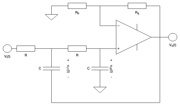
Explaining how to apply circuit analysis is way out of scope for this blog. But one set of equations that describes the circuit in the Laplace domain is given below:
\[ \begin{array}{rl} sV_{c1}(s) &= \frac{-2V_{c1}(s) - \frac{R_b+2R_q}{R_b}V_{c2}(s)}{RC} + \frac{V_i(s)}{RC} \\ sV_{c2}(s) &= \frac{V_{c1}(s) + \frac{R_q}{R_b}V_{c2}(s)}{RC} \\ V_o(s) &= \frac{R_b+R_q}{R_b} V_{c2}(s) \end{array} \]
Before we go further, we will make some substitutions in the above equations to simplify further working. Define \(k=\frac{R_q}{R_b}\) and \(\omega=\frac{1}{RC}\) to get:
\[ \begin{array}{rl} sV_{c1}(s) &= -2 \omega V_{c1}(s) - \left(2k+1\right)\omega V_{c2}(s) + \omega V_i(s) \\ sV_{c2}(s) &= \omega V_{c1}(s) + k \omega V_{c2}(s) \\ V_o(s) &= \left(k+1\right) V_{c2}(s) \end{array} \]
At this point, we can do some substitution of the equations above to find \(\frac{V_o(s)}{V_i(s)}\) i.e. the unique transfer function of the circuit:
\[ \frac{V_o(s)}{V_i(s)} = \frac{\omega^2}{s^2 + s\omega(2-k) + \omega^2}(k+1) \]
This looks very similar to the resonant lowpass function given previosuly with \(Q=\frac{1}{2-k}\) and an additional gain of \(k+1\) tacked on.
Given that there are no common components in determining \(\omega\) and \(k\), the analogue VCVS filter topology has the ability to provide independent control of \(Q\) and \(\omega\) (although, the overall gain of the system is affected by \(Q\)).
We've stated what we want: the states to approximate the voltages across the capacitors. We know that we cannot do that if we use a standard difference equation obtained via a transfer function. So what next?
Straight to state-space
We derived the equations for the analogue model carefully in the previous section. We ensured that the \(s\) terms only existed on the left hand side and only multiplied each of the states we said we were interested in. This enables us to write out the state-space model directly as follows:
\[ \begin{array}{rll} s \left[ \begin{array}{c} V_{c1}(s) \\ V_{c2}(s) \end{array} \right] &= \left[ \begin{array}{cc} -2\omega & -\left(2k+1\right)\omega \\ \omega & k\omega \end{array} \right] \left[ \begin{array}{c} V_{c1}(s) \\ V_{c2}(s) \end{array} \right] & + \left[ \begin{array}{c} \omega \\ 0 \end{array} \right] V_i(s) \\ V_o(s) &= \left[ \begin{array}{c} 0 & k+1 \end{array} \right] \left[ \begin{array}{c} V_{c1}(s) \\ V_{c2}(s) \end{array} \right] &+ 0 V_i(s) \end{array} \]
If we define the state vector \(\mathbf{Q}(s) = \left[ \begin{array}{cc} V_{c1}(s) & V_{c2}(s) \end{array} \right]^T\), the input vector \(\mathbf{X}(s)=V_i(s)\) and the output vector \(\mathbf{Y}(s)=V_o(s)\) we can write the above in the usual state variable representation:
\[ \begin{array}{rll} s \mathbf{Q}(s) &= \mathbf{A} \mathbf{Q}(s) + \mathbf{B} \mathbf{X}(s) \\ \mathbf{Y}(s) &= \mathbf{C} \mathbf{Q}(s) + \mathbf{D} \mathbf{X}(s) \end{array} \]
The top equation is the state equation. The bottom is the output equation. Recall that the state-space mapping is not unique. We can change the coordinates of the \(\mathbf{Q}(s)\) vector using any invertible matrix as demonstrated in the state-space primer post. But here, we have intentionally chosen the states we want to use so that our system behaves similarly to the circuit. What we will now do is apply the bilinear transform to this system in such a way that our output equation remains the same as in the continuous system - which it must if we are actually modelling the circuit. Defining the bilinear transform as:
\[ s=\alpha\frac{z-1}{z+1} \]
Where \(\alpha\) is related to the sampling rate of the system we are building and can be used to control the specific frequency in the frequency response that maps exactly to the \(s\)-domain transfer function (see the wikipedia page for the bilinear transform for more information). Make the substitution to the state update equation and attempt to make the left hand side \(z\mathbf{Q}(z)\):
\[ \normalsize \begin{array}{rl} \alpha\frac{z-1}{z+1} \mathbf{Q}(z) &= \mathbf{A} \mathbf{Q}(z) + \mathbf{B} \mathbf{X}(z) \\ \alpha\left(z-1\right) \mathbf{Q}(z) &= \left(z+1\right) \mathbf{A}\mathbf{Q}(z) + \left(z+1\right) \mathbf{B} \mathbf{X}(z) \\ z\left(\alpha\mathbf{I}-\mathbf{A}\right)\mathbf{Q}(z) &= \left(\mathbf{\alpha \mathbf{I} + A}\right) \mathbf{Q}(z) + \left(z+1\right) \mathbf{B} \mathbf{X}(z) \\ z\mathbf{Q}(z) &= \left(\alpha\mathbf{I}-\mathbf{A}\right)^{-1}\left(\mathbf{\alpha \mathbf{I} + A}\right) \mathbf{Q}(z) + \left(z+1\right) \left(\alpha\mathbf{I}-\mathbf{A}\right)^{-1}\mathbf{B} \mathbf{X}(z) \end{array} \]
Note that the input mixing term includes \((z+1)\). Normally, this term would be moved into the output equation (so that it can be eliminated) and would cause the \(\mathbf{C}\) and \(\mathbf{D}\) matrices to change indicating that we have changed the states - but we don't want this! Instead, we simply implement that operation on the input before mixing it.
The only thing that remains is to make the system causal i.e. the system has the following form:
\[ \begin{array}{rll} z \mathbf{Q}(z) &= \mathbf{A_d} \mathbf{Q}(z) + \left(z+1\right)\mathbf{B_d} \mathbf{X}(z) \\ \mathbf{Y}(z) &= \mathbf{C} \mathbf{Q}(z) + \mathbf{D} \mathbf{X}(z) \end{array} \]
This depends on future samples of \(\mathbf{X}(z)\). We multiply the state update equation by \(z^{-1}\) to get:
\[ \begin{array}{rll} \mathbf{Q}(z) &= z^{-1} \mathbf{A_d} \mathbf{Q}(z) + \left(1+z^{-1}\right)\mathbf{B_d} \mathbf{X}(z) \\ \mathbf{Y}(z) &= \mathbf{C} \mathbf{Q}(z) + \mathbf{D} \mathbf{X}(z) \end{array} \]
Converting this into a state-space difference-equation we get:
\[ \begin{array}{rll} \mathbf{Q}[n] &= \mathbf{A_d} \mathbf{Q}[n-1] + \mathbf{B_d}\left(\mathbf{X}[n] + \mathbf{X}[n-1]\right) \\ \mathbf{Y}[n] &= \mathbf{C} \mathbf{Q}[n] + \mathbf{D} \mathbf{X}[n] \end{array} \]
The above is what we implement. \(\mathbf{C}\) and \(\mathbf{D}\) are the same as what we derived for our continuous time system (\(\mathbf{C}=\left[\begin{array}{cc}0 & k+1 \end{array}\right]\) and \(\mathbf{D}=0\)). \(\mathbf{A_d}\) and \(\mathbf{B_d}\) are defined as:
\[ \begin{array}{rl} \mathbf{A_d} &= \left(\alpha\mathbf{I}-\mathbf{A}\right)^{-1}\left(\mathbf{\alpha \mathbf{I} + A}\right) \\ \mathbf{B_d} &= \left(\alpha\mathbf{I}-\mathbf{A}\right)^{-1}\mathbf{B} \end{array} \]
Making it more useful
If we stopped here, we would have the lowpass filter the circuit represented. But who just wants a lowpass filter?
Based on how we designed the system earlier, all the properties of the circuit are modeled by the \(\mathbf{A_d}\) and \(\mathbf{B_d}\) matrices. The \(\mathbf{C}\) and \(\mathbf{D}\) matrices can be thought of as buffering values available at various points in the circuit and mixing them with various gains to create the output i.e. the \(\mathbf{C}\) and \(\mathbf{D}\) matrices can be thought to not really impact the circuit - only how the output is tapped from it. If we let \(\mathbf{C}=\left[\begin{array}{cc}c0&c1\end{array}\right]\) and \(\mathbf{D}=d_0\) and expand the analogue transfer function, we get:
\[ \begin{array}{rll} \mathbf{A} &= \left[ \begin{array}{cc} -2\omega & -\left(2k+1\right)\omega \\ \omega & k\omega \end{array} \right] \\ \mathbf{B} &= \left[ \begin{array}{c} \omega \\ 0 \end{array} \right] \\ \frac{V_o(s)}{V_i(s)} &= \mathbf{C}(s\mathbf{I} - \mathbf{A})^{-1}\mathbf{B} + d_0 \\ &= \frac{\mathbf{C} ( \text{adj } s\mathbf{I}-\mathbf{A})\mathbf{B}}{\det s\mathbf{I} - \mathbf{A}} + d_0 \\ &= \frac{\left[\begin{array}{cc}c_0 & c_1\end{array}\right]\left[\begin{array}{cc} s - k\omega & -(2k+1)\omega \\ \omega & s+2\omega \end{array} \right] \left[\begin{array}{c} \omega \\ 0\end{array} \right]}{s^2 +s\omega(2-k) +\omega^2} + d_0 \\ &= \frac{d_0 s^2+s\omega(c_0 +d_0 (2-k))+\omega^2(d_0+c_1-c_0k)}{s^2 +s\omega(2-k) +\omega^2} \end{array} \]
We can use \(d_0\), \(c_0\) and \(c_1\) to create any numerator of our choosing. The denominator is completely determined by the \(\mathbf{A}\) matrix, but recall the list of resonant filters at the start of this post also share the same denominator. We can use this information to build multiple outputs from the same states and input sample! We can even build some smooth control to transition between them. Let's try obtain these quantities from something a bit more readable:
\[ d_0 s^2+s\omega(c_0 +d_0 (2-k))+\omega^2(d_0+c_1-c_0k) = b_2 s^2 + s\omega b_1 + b_0\omega^2 \]
Solving for \(d_0\), \(c_0\) and \(c_1\):
\[ \begin{array}{rl} d_0 &= b_2 \\ c_0 &= b_1 - (2-k)b_2 \\ c_1 &= b_0-d_0+c_0k = b_0 + k b_1 - (k(2-k)+1)b_2\end{array} \]
- Setting \(b_2=0\), \(b_1=0\) and \(b_0=1\) makes the resonant lowpass filter.
- Setting \(b_2=1\), \(b_1=0\) and \(b_0=0\) makes the resonant highspass filter.
- Setting \(b_2=1\), \(b_1=g(2-k)\) and \(b_0=1\) makes the resonant bandpass/bandstop filter dependent on the value of \(g\).
We could introduce a parameter \(p\) to transition between lowpass and highpass as follows:
\[ \begin{array}{rl} b_0 &= 1-p \\ b_1 &= 0 \\ b_2 &= p\end{array} \]
When \(p=0\), the system is lowpass. When \(p=1\), the system is highpass. When \(p=0.5\), we have a bandstop filter with a wideband attenuation of 6 dB. That's kinda funky, but it would be cool if we could hack in some controllable bandpass/bandstop behaviour too. We can fudge this by setting:
\[ \begin{array}{rl} b_0 &= 1-p \\ b_1 &= 2(1-p)p(2-k)g \\ b_2 &= p\end{array} \]
Now when \(p=0.5\) we have a controllable bandpass/bandstop filter dependent on the value of \(g\).
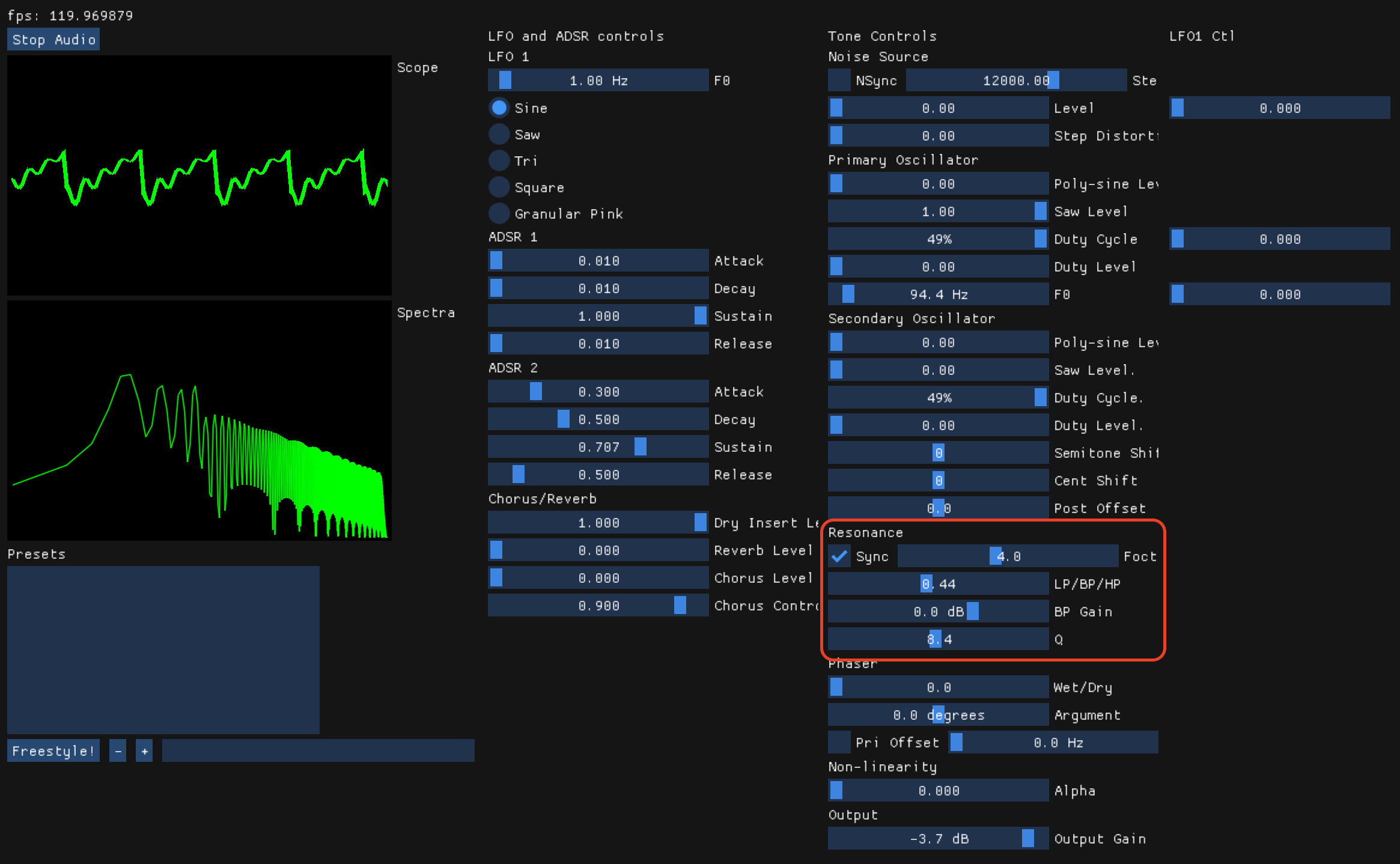
The “Sync” checkbox controls whether \(\omega\) should be:
- If unchecked, a constant. The slider next to it will be in Hz.
- If checked, a multiple of the main oscillator frequency.
The “LP/BP/HP” slider directly controls \(p\). \(g\) gets the linear gain corresponding to the value of “BP Gain”. The value of the “Q” slider is converted to \(k\) as described earlier.
Summary of implementation
The implementation has 4 input parameters:
- \(p\) is the continuous mode control. It is in the range [0, 1]. At 0, the system is lowpass. At 1, the system is highpass. At 0.5, the system is bandpass/bandstop.
- \(g\) is the linear bandpass/bandstop gain. When \(p=0\) and \(g=0\), the system is bandstop. When \(p=0\) and \(g=1\), the output is the input. When \(p=0.5\) and \(g\gg1\), the system is bandboost.
- \(\omega\) the natural frequency of the filter - this will be close to where resonance occurs.
- \(k\) the derived from the Q-factor.
For every sample:
- Smooth the control parameters \(p\), \(g\), \(\omega\), \(k\) with 1-pole smoothers to avoid instantaneous jumps which will cause glitches.
- Form the \(\mathbf{A}\) and \(\mathbf{B}\) matrices and compute their discretised counterparts as described (yes, this is an entire bilinear transform per sample).
- Evaluate the state update equation to form the new states.
- Derive \(\mathbf{C}\) and \(\mathbf{D}\) using: \[ \begin{array}{rl} b_0 &= 1-p \\ b_1 &= 2(1-p)p(2-k)g \\ b_2 &= p\end{array} \]
- Evaluate the output equation to get the next output sample.